Ray is an open-source unified compute framework that simplifies scaling AI and Python workloads in a distributed atmosphere. Since we launched assist for operating Ray on Databricks, we have witnessed quite a few clients efficiently deploying their machine studying use instances, which vary from forecasting and deep reinforcement studying to fine-tuning LLMs.

With the discharge of Ray model 2.8.0, we’re delighted to announce the addition of autoscaling assist for Ray on Databricks. Autoscaling is crucial as a result of it permits assets to dynamically regulate to fluctuating calls for. This ensures optimum efficiency and cost-efficiency, as processing wants can range considerably over time, and it helps keep a stability between computational energy and bills with out requiring handbook intervention.

Ray autoscaling on Databricks can add or take away employee nodes as wanted, leveraging the Spark framework to boost scalability, cost-effectiveness, and responsiveness in distributed computing environments. This built-in method is much less complicated than the choice of implementing OSS autoscaling by eliminating the necessity for outlining advanced permissions, cloud initialization scripts, and logging configurations. With a fully-managed, production-capable, and built-in autoscaling resolution, you possibly can vastly cut back the complexity and price of your Ray workloads.

Create Ray cluster on Databricks with autoscaling enabled

To get began, merely set up the newest model of Ray

# Set up Ray with the 'default','tune' extensions for
# Ray dashboard, and tuning assist
%pip set up ray[default,tune]>=2.8.0

The subsequent step is to ascertain the configuration for the Ray cluster that we will be beginning through the use of the `ray.util.spark.setup_ray_cluster() ` operate. So as to leverage autoscaling performance, specify the utmost variety of employee nodes that the Ray cluster can use, outline the allotted compute assets, and set the Autoscale flag to True. Moreover, it’s essential to make sure that the Databricks cluster has been began with autoscaling enabled. For extra particulars, please check with the documentation.

As soon as these parameters have been set, while you initialize the Ray cluster, autoscaling will operate precisely as Databricks autoscaling does. Under is an instance of establishing a Ray cluster with the flexibility to autoscale.

from ray.util.spark import setup_ray_cluster
setup_ray_cluster(
 num_worker_nodes,#set to max variety of nodes to Autoscale  
 num_cpus_head_node,# set to the cores used within the driver node
 num_gpus_head_node, # set for GPU enabled cluster
 num_cpus_per_node,# cores added from every employee node
 num_gpus_per_node, #set for GPU enabled cluster
 autoscale = True #set just for clusters with Auto Scaling Enabled
)

This function is suitable with any Databricks cluster operating Databricks Runtime model 14.0 or above.

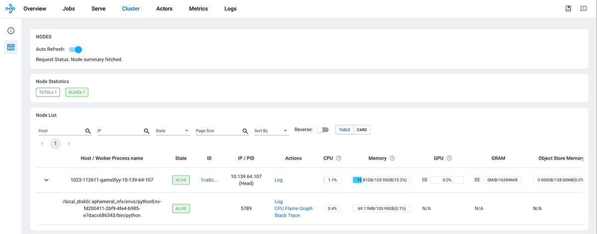
To study extra concerning the parameters which might be out there for configuring a Ray cluster on Spark, please check with the setup_ray_cluster documentation. As soon as the Ray cluster is initialized, the Ray head node will present up on the Ray Dashboard.

from ray.util.spark import setup_ray_cluster, shutdown_ray_cluster

ray_conf = setup_ray_cluster(
     num_worker_nodes= 4,
     num_cpus_head_node=3,
     num_cpus_per_node=4,
     autoscale = True
)

When a job is submitted to the Ray cluster, the Ray Autoscaler API requests assets from the Spark cluster by submitting duties with the mandatory CPU and GPU compute necessities. The Spark scheduler scales up employee nodes if the present cluster assets can’t meet the duty’s compute calls for and scales down the cluster when duties are accomplished and no extra duties are pending. You’ll be able to management the scale-up and scale-down velocity by adjusting the autoscale_upscaling_speed and autoscale_idle_timeout_minutes parameters. For added particulars about these management parameters, please check with the documentation. As soon as the method is accomplished, Ray releases all the allotted assets again to the Spark cluster for different duties or for downscaling, making certain environment friendly utilization of assets.

Let’s stroll by means of a hyperparameter tuning instance to display the autoscaling course of. On this instance, we’ll practice a PyTorch mannequin on the CIFAR10 dataset. We have tailored the code from the Ray documentation, which you could find right here.

We’ll start by defining the PyTorch mannequin we need to tune.

import torch.nn as nn
import torch.nn.useful as F


class Internet(nn.Module):
 def __init__(self, l1=120, l2=84):
  tremendous(Internet, self).__init__()
  self.conv1 = nn.Conv2d(3, 6, 5)
  self.pool = nn.MaxPool2d(2, 2)
  self.conv2 = nn.Conv2d(6, 16, 5)
  self.fc1 = nn.Linear(16 * 5 * 5, l1)
  self.fc2 = nn.Linear(l1, l2)
  self.fc3 = nn.Linear(l2, 10)

 def ahead(self, x):
  x = self.pool(F.relu(self.conv1(x)))
  x = self.pool(F.relu(self.conv2(x)))
  x = x.view(-1, 16 * 5 * 5)
  x = F.relu(self.fc1(x))
  x = F.relu(self.fc2(x))
  x = self.fc3(x)
  return x

We wrap the information loaders in their very own operate and cross a worldwide knowledge listing. This fashion we will share an information listing between totally different trials.

import torchvision
import torchvision.transforms as transforms
from filelock import FileLock


def load_data(data_dir="./knowledge"):
    rework = transforms.Compose(
        [transforms.ToTensor(), transforms.Normalize((0.5, 0.5, 0.5), (0.5, 0.5, 0.5))]
    )

    # We add FileLock right here as a result of a number of staff will need to
    # obtain knowledge, and this will likely trigger overwrites since
    # DataLoader is just not threadsafe.
    with FileLock(os.path.expanduser("~/.knowledge.lock")):
        trainset = torchvision.datasets.CIFAR10(
            root=data_dir, practice=True, obtain=True, rework=rework
        )

        testset = torchvision.datasets.CIFAR10(
            root=data_dir, practice=False, obtain=True, rework=rework
        )

    return trainset, testset

Subsequent, we will outline a operate that may ingest a config and run a single coaching loop for the torch mannequin. On the conclusion of every trial, we checkpoint the weights and report the evaluated loss utilizing the `practice, report` API. That is completed in order that the scheduler can cease ineffectual trials that don’t enhance the mannequin’s loss traits.

import os
import torch
import torch.optim as optim
from torch.utils.knowledge import random_split

import ray
from ray import practice, tune
from ray.practice import Checkpoint


def train_cifar(config, loc):  # location to retailer the checkpoints
    internet = Internet(config["l1"], config["l2"])
    # test whether or not to load in CPU or GPU
    system = "cpu"
    if torch.cuda.is_available():
        system = "cuda:0"
    internet.to(system)

    criterion = nn.CrossEntropyLoss()
    optimizer = optim.SGD(internet.parameters(), lr=config["lr"], momentum=0.9)

    # load the Dataset
    data_dir = os.path.abspath("./knowledge")
    trainset, testset = load_data(data_dir)

    test_abs = int(len(trainset) * 0.8)
    train_subset, val_subset = random_split(
        trainset, [test_abs, len(trainset) - test_abs]
    )

    trainloader = torch.utils.knowledge.DataLoader(
        train_subset, batch_size=int(config["batch_size"]), shuffle=True, num_workers=8
    )
    valloader = torch.utils.knowledge.DataLoader(
        val_subset, batch_size=int(config["batch_size"]), shuffle=True, num_workers=8
    )

Subsequent, we outline the coaching loop which runs for the full epochs specified within the config file, Every epoch consists of two most important components:

• The Prepare Loop – iterates over the coaching dataset and tries to converge to optimum parameters.
• The Validation/Take a look at Loop – iterates over the take a look at dataset to test if mannequin efficiency is bettering.

for epoch in vary(config["max_epoch"]):  # loop over the dataset a number of instances
    running_loss = 0.0
    epoch_steps = 0
    for i, knowledge in enumerate(trainloader, 0):
        # get the inputs; knowledge is a listing of [inputs, labels]
        inputs, labels = knowledge
        inputs, labels = inputs.to(system), labels.to(system)

        # zero the parameter gradients
        optimizer.zero_grad()

        # ahead + backward + optimize
        outputs = internet(inputs)
        loss = criterion(outputs, labels)
        loss.backward()
        optimizer.step()

        # print statistics
        running_loss += loss.merchandise()
        epoch_steps += 1
        if i % 2000 == 1999:  # print each 2000 mini-batches
            print(
                "[%d, %5d] loss: %.3f" % (epoch + 1, i + 1, running_loss / epoch_steps)
            )
            running_loss = 0.0

        # Validation loss
        val_loss = 0.0
        val_steps = 0
        complete = 0
        right = 0
        for i, knowledge in enumerate(valloader, 0):
            with torch.no_grad():
                inputs, labels = knowledge
                inputs, labels = inputs.to(system), labels.to(system)
                outputs = internet(inputs)
                _, predicted = torch.max(outputs.knowledge, 1)
                complete += labels.measurement(0)
                right += (predicted == labels).sum().merchandise()
                loss = criterion(outputs, labels)
                val_loss += loss.cpu().numpy()
                val_steps += 1

Lastly, we first save a checkpoint after which report some metrics again to Ray Tune. Particularly, we ship the validation loss and accuracy again to Ray Tune. Ray Tune can then use these metrics to resolve which hyperparameter configuration results in one of the best outcomes.

# Right here we save a checkpoint. It's routinely registered with
# Ray Tune and could be accessed by means of `practice.get_checkpoint()`
# API in future iterations.
import os
import torch
import ray
from ray import practice
from ray.practice import Checkpoint

os.makedirs(f"{loc}/mymodel", exist_ok=True)
torch.save((internet.state_dict(), optimizer.state_dict()), f"{loc}/mymodel/checkpoint.pt")
checkpoint = Checkpoint.from_directory(f"{loc}/mymodel/")
practice.report(
    {"loss": (val_loss / val_steps), "try_gpu": False, "accuracy": right / complete},
    checkpoint=checkpoint,
)
print("Completed Coaching")

Subsequent, we outline the primary elements to start out the tuning job by specifying the search area that the optimizer will choose from for given hyperparameters.

Outline the search area

The configuration under expresses the hyperparameters and their search choice ranges as a dictionary. For every of the given parameter varieties, we use the suitable selector algorithm (i.e., sample_from, loguniform, or alternative, relying on the character of the parameter being outlined).

from ray import tune
config = {
   "l1": tune.sample_from(lambda _: 2 ** np.random.randint(2, 9)),
   "l2": tune.sample_from(lambda _: 2 ** np.random.randint(2, 9)),
   "lr": tune.loguniform(1e-4, 1e-1),
   "batch_size": tune.alternative([2, 4, 8, 16]),
   "max_epoch":20
}

At every trial, Ray Tune will randomly pattern a mix of parameters from these search areas. After choosing a worth for every of the parameters throughout the confines of our configuration that we outlined above, it would then practice plenty of fashions in parallel in an effort to discover the best-performing one among the many group. So as to short-circuit an iteration of parameter choice that is not working effectively, we use the ASHAScheduler, which is able to terminate ineffective trials early i.e. trials whose loss metrics are considerably degraded in comparison with the present best-performing set of parameters from the run’s historical past.

from ray.tune.schedulers import ASHAScheduler

scheduler = ASHAScheduler(
   max_t=config['max_epoch'],
   grace_period=5,
   reduction_factor=2
)

Tune API

Lastly, we name the Tuner API to provoke the run. When calling the coaching initiating methodology, we cross some extra configuration choices that outline the assets that we allow Ray Tune to make use of per trial, the default storage location of checkpoints, and the goal metric to optimize throughout the iterative optimization. Refer right here for extra particulars on the assorted parameters which might be out there for Ray Tune.

import os
from ray import practice, tune

tuner = tune.Tuner(
    tune.with_resources(
        tune.with_parameters(train_cifar, loc=loc),
        assets={"cpu": cpus_per_trial, "gpu": gpus_per_trial},
    ),
    tune_config=tune.TuneConfig(
        metric="loss",
        mode="min",
        scheduler=scheduler,
        num_samples=num_samples,  # complete trails to run given the search area
    ),
    run_config=practice.RunConfig(
        storage_path=os.path.expanduser(loc), title="tune_checkpointing_location"
    ),
    param_space=config,
)

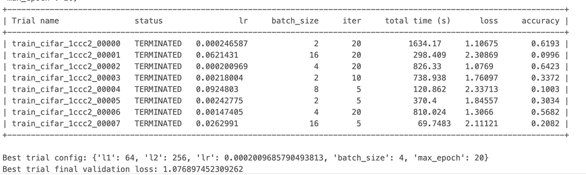
outcomes = tuner.match()

So as to see what occurs after we run this code with a selected declared useful resource constraint, let’s set off the run with CPU solely, utilizing cpus_per_trial = 3 and gpu = 0 with total_epochs = 20 for the run configuration.

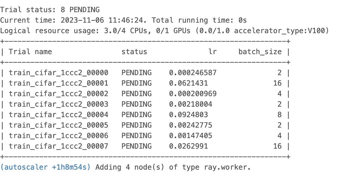
We see the autoscaler begin requesting assets as proven above and the pending useful resource logged within the UI proven under.

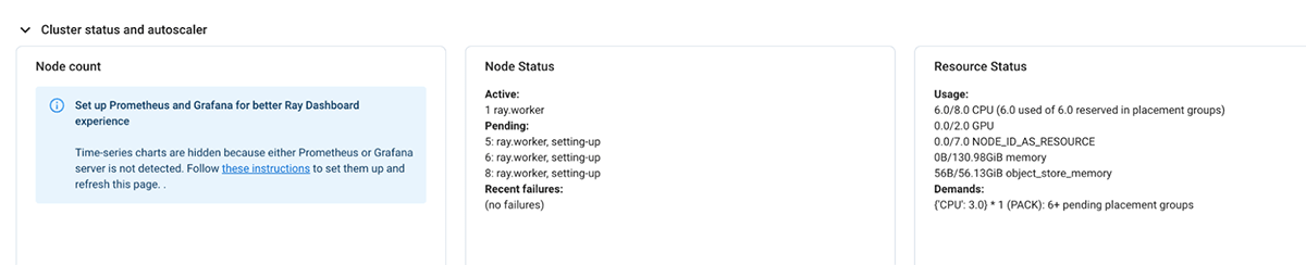
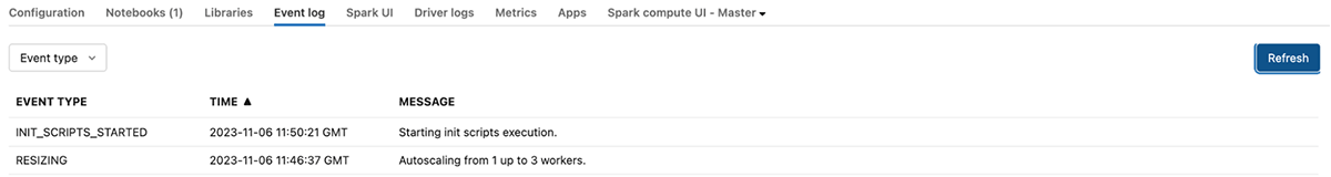
If the present demand for assets by the Ray cluster can’t be met, it initiates autoscaling of the databricks cluster as effectively.

Lastly, we will see the run finishes the output of the Job exhibits that among the dangerous trials have been terminated early resulting in compute financial savings

The identical course of works with none code change with GPU assets as effectively with none code change. Be happy to clone the pocket book and run it in your atmosphere:

What’s subsequent

With the assist for autoscaling Ray workload, we take one step additional to tighten the mixing between Ray and Databricks and assist scale your dynamic workloads. Our roadmap for this integration guarantees much more thrilling developments. Keep tuned for additional updates!